← Back to Insights

Teaching Note

Imposing and Testing Zero-Degree Homogeneity in Demand1

Python and R replication code · Practical README

1. Intuition and a numerical example

A household with a monthly income of €2,000 chooses a basket. Suppose every price and its income double. A basket xx was affordable before if p⋅x≤2000p\cdot x\le 2000⁠; it is affordable now if 2p⋅x≤40002p\cdot x\le 4000⁠, which is the same inequality. The budget set has not moved, so a household that cares about quantities, not about nominal values, has no reason to change its basket. Demand is homogeneous of degree zero in prices and income: this is the formal definition of “no money illusion”.

The econometrician observes JJ prices and income YY and writes the demand for good 1 as

log⁡q1=β0+∑j=1Jβjlog⁡pj+βJ+1log⁡Y+u.(1)\log q_1=\beta_0+\sum_{j=1}^{J}\beta_j\log p_j+\beta_{J+1}\log Y+u . \qquad \htmlId{equation-1}{(1)}

Section 3 shows that multiplying all prices and income by λ>0\lambda>0 multiplies q1q_1 by λθ\lambda^{\theta}⁠, where θ≡∑j=1Jβj+βJ+1\theta\equiv\sum_{j=1}^J\beta_j+\beta_{J+1}⁠. With θ=0.1\theta=0.1⁠, doubling prices and income raises demand by 20.1−1=7.2%2^{0.1}-1=7.2\%⁠, although nothing real has changed: that is money illusion. Homogeneity is the restriction θ=0\theta=0⁠.

2. From the utility function to the demand function

The general result. The Marshallian demand x(p,Y)x(p,Y) maximises U(x)U(x) over the budget set B(p,Y)={x≥0: p⋅x≤Y}B(p,Y)=\{x\ge0:\ p\cdot x\le Y\}⁠. (I write UU for utility and keep uu for the error term.) For any λ>0\lambda>0⁠:

B(λp,λY)={x≥0: (λp)⋅x≤λY}={x≥0: λ (p⋅x)≤λY}={x≥0: p⋅x≤Y}(divide by λ>0)=B(p,Y),x(λp,λY)=arg⁡max⁡x∈B(λp,λY)U(x)=arg⁡max⁡x∈B(p,Y)U(x)=x(p,Y).(2)\begin{aligned} B(\lambda p,\lambda Y)&=\{x\ge0:\ (\lambda p)\cdot x\le \lambda Y\} \\ &=\{x\ge0:\ \lambda\,(p\cdot x)\le \lambda Y\} \\ &=\{x\ge0:\ p\cdot x\le Y\}\qquad\text{(divide by }\lambda>0) \\ &=B(p,Y), \\ x(\lambda p,\lambda Y)&=\arg\max_{x\in B(\lambda p,\lambda Y)}U(x)=\arg\max_{x\in B(p,Y)}U(x)=x(p,Y). && \htmlId{equation-2}{(2)} \end{aligned}

Homogeneity is therefore a consequence of the budget constraint, not an assumption about the shape of preferences. It requires only that UU depends on quantities and not on nominal magnitudes, and that the maximiser is unique (otherwise the demand set is homogeneous).

Cobb–Douglas. Let U(x)=∑jαjlog⁡xjU(x)=\sum_j\alpha_j\log x_j with αj>0\alpha_j>0 and ∑jαj=1\sum_j\alpha_j=1⁠. The budget constraint binds because UU is increasing.

L=∑j=1Jαjlog⁡xj−μ(∑j=1Jpjxj−Y)(3)∂L∂xj=αjxj−μpj=0,j=1,…,J(4)∂L∂μ=0 ⟺ ∑j=1Jpjxj=Y(5)from (4):pjxj=αjμ,j=1,…,J(6)sum (6) over j:∑j=1Jpjxj=1μ∑j=1Jαj=1μuse (5):Y=1μ⟹μ=1Yput μ=1/Y in (6), j=1:p1x1=α1Yx1=α1Yp1(7)log⁡x1=log⁡α1−log⁡p1+log⁡Y.(8)\begin{aligned} \mathcal L&=\sum_{j=1}^J\alpha_j\log x_j-\mu\Big(\sum_{j=1}^Jp_jx_j-Y\Big) && \htmlId{equation-3}{(3)} \\ \frac{\partial\mathcal L}{\partial x_j}&=\frac{\alpha_j}{x_j}-\mu p_j=0,\qquad j=1,\dots,J && \htmlId{equation-4}{(4)} \\ \frac{\partial\mathcal L}{\partial \mu}&=0\ \Longleftrightarrow\ \sum_{j=1}^Jp_jx_j=Y && \htmlId{equation-5}{(5)} \\ \text{from (4):}\quad p_jx_j&=\frac{\alpha_j}{\mu},\qquad j=1,\dots,J && \htmlId{equation-6}{(6)} \\ \text{sum (6) over } j:\quad \sum_{j=1}^Jp_jx_j&=\frac1\mu\sum_{j=1}^J\alpha_j=\frac1\mu \\ \text{use (5):}\quad Y&=\frac1\mu\quad\Longrightarrow\quad \mu=\frac1Y \\ \text{put }\mu=1/Y\text{ in (6), }j=1:\quad p_1x_1&=\alpha_1Y \\ x_1&=\frac{\alpha_1Y}{p_1} && \htmlId{equation-7}{(7)} \\ \log x_1&=\log\alpha_1-\log p_1+\log Y. && \htmlId{equation-8}{(8)} \end{aligned}

Comparing (8) with (1): β0=log⁡α1\beta_0=\log\alpha_1⁠, β1=−1\beta_1=-1⁠, βj=0\beta_j=0 for j=2,…,Jj=2,\dots,J⁠, βJ+1=1\beta_{J+1}=1⁠, so θ=−1+0+1=0\theta=-1+0+1=0⁠. Directly on (7):

x1(λp,λY)=α1 λYλp1=α1Yp1=x1(p,Y).x_1(\lambda p,\lambda Y)=\frac{\alpha_1\,\lambda Y}{\lambda p_1}=\frac{\alpha_1Y}{p_1}=x_1(p,Y).

Stone–Geary (linear expenditure system). Cobb–Douglas forces zero cross-price elasticities and a unit income elasticity. Let instead U(x)=∑jαjlog⁡(xj−γj)U(x)=\sum_j\alpha_j\log(x_j-\gamma_j)⁠, with αj>0\alpha_j>0⁠, ∑jαj=1\sum_j\alpha_j=1⁠, xj>γjx_j>\gamma_j and Y>∑jpjγjY>\sum_jp_j\gamma_j (Stone, 1954). The Lagrangian is the same as (3) with log⁡(xj−γj)\log(x_j-\gamma_j) in place of log⁡xj\log x_j⁠; the condition ∂L/∂μ=0\partial\mathcal L/\partial\mu=0 is again (5).

∂L∂xj=αjxj−γj−μpj=0,j=1,…,J(9)from (9):pjxj=pjγj+αjμ,j=1,…,J(10)sum (10) over j, use (5) and ∑jαj=1:Y=∑j=1Jpjγj+1μ1μ=Y−∑j=1Jpjγj(11)put (11) in (10), j=1:p1x1=p1γ1+α1(Y−∑j=1Jpjγj)x1=γ1+α1p1(Y−∑j=1Jpjγj).(12)\begin{aligned} \frac{\partial\mathcal L}{\partial x_j}&=\frac{\alpha_j}{x_j-\gamma_j}-\mu p_j=0,\qquad j=1,\dots,J && \htmlId{equation-9}{(9)} \\ \text{from (9):}\quad p_jx_j&=p_j\gamma_j+\frac{\alpha_j}{\mu},\qquad j=1,\dots,J && \htmlId{equation-10}{(10)} \\ \text{sum (10) over } j\text{, use (5) and }\textstyle\sum_j\alpha_j=1:\quad Y&=\sum_{j=1}^Jp_j\gamma_j+\frac1\mu \\ \frac1\mu&=Y-\sum_{j=1}^Jp_j\gamma_j && \htmlId{equation-11}{(11)} \\ \text{put (11) in (10), }j=1:\quad p_1x_1&=p_1\gamma_1+\alpha_1\Big(Y-\sum_{j=1}^Jp_j\gamma_j\Big) \\ x_1&=\gamma_1+\frac{\alpha_1}{p_1}\Big(Y-\sum_{j=1}^Jp_j\gamma_j\Big). && \htmlId{equation-12}{(12)} \end{aligned}

The multiplier is the inverse of supernumerary income (11); the household buys the committed quantity γ1\gamma_1 and spends a share α1\alpha_1 of what is left (12). Homogeneity, directly on (12):

x1(λp,λY)=γ1+α1λp1(λY−∑j=1Jλpjγj)=γ1+λ α1λ p1(Y−∑j=1Jpjγj)=x1(p,Y).\begin{aligned} x_1(\lambda p,\lambda Y)&=\gamma_1+\frac{\alpha_1}{\lambda p_1}\Big(\lambda Y-\sum_{j=1}^J\lambda p_j\gamma_j\Big) =\gamma_1+\frac{\lambda\,\alpha_1}{\lambda\,p_1}\Big(Y-\sum_{j=1}^Jp_j\gamma_j\Big)=x_1(p,Y). \end{aligned}

Elasticities. Differentiate (12); for the own price, use (12) in the form (α1/p1)(Y−∑jpjγj)=x1−γ1(\alpha_1/p_1)(Y-\sum_jp_j\gamma_j)=x_1-\gamma_1⁠:

∂x1∂Y=α1p1⟹η1=Yx1∂x1∂Y=α1Yp1x1∂x1∂pj=−α1γjp1 (j≠1)⟹ε1j=pjx1∂x1∂pj=−α1γjpjp1x1∂x1∂p1=−α1p12(Y−∑jpjγj)−α1γ1p1=−x1−γ1+α1γ1p1⟹ε11=−1+(1−α1)γ1x1.(13)\begin{aligned} \frac{\partial x_1}{\partial Y}=\frac{\alpha_1}{p_1} \quad&\Longrightarrow\quad \eta_1=\frac{Y}{x_1}\frac{\partial x_1}{\partial Y}=\frac{\alpha_1Y}{p_1x_1} \\ \frac{\partial x_1}{\partial p_j}=-\frac{\alpha_1\gamma_j}{p_1}\ (j\ne1) \quad&\Longrightarrow\quad \varepsilon_{1j}=\frac{p_j}{x_1}\frac{\partial x_1}{\partial p_j}=-\frac{\alpha_1\gamma_jp_j}{p_1x_1} \\ \frac{\partial x_1}{\partial p_1}=-\frac{\alpha_1}{p_1^2}\Big(Y-\sum_{j}p_j\gamma_j\Big)-\frac{\alpha_1\gamma_1}{p_1}=-\frac{x_1-\gamma_1+\alpha_1\gamma_1}{p_1} \quad&\Longrightarrow\quad \varepsilon_{11}=-1+\frac{(1-\alpha_1)\gamma_1}{x_1}. && \htmlId{equation-13}{(13)} \end{aligned}

Cross-price elasticities are non-zero as soon as γj≠0\gamma_j\ne0 (negative when γj>0\gamma_j>0), and η1≠1\eta_1\ne1 unless γ=0\gamma=0⁠. Their sum, over the common denominator p1x1p_1x_1⁠:

p1x1(∑j=1Jε1j+η1)=[−p1x1+(1−α1)p1γ1]−α1∑j≠1pjγj+α1Y=−p1x1+p1γ1+α1(Y−∑j=1Jpjγj)=−p1x1+p1x1=0by (12).\begin{aligned} p_1x_1\Big(\sum_{j=1}^J\varepsilon_{1j}+\eta_1\Big) &=\big[-p_1x_1+(1-\alpha_1)p_1\gamma_1\big]-\alpha_1\sum_{j\ne1}p_j\gamma_j+\alpha_1Y \\ &=-p_1x_1+p_1\gamma_1+\alpha_1\Big(Y-\sum_{j=1}^Jp_j\gamma_j\Big) \\ &=-p_1x_1+p_1x_1=0\qquad\text{by (12).} \end{aligned}

Numerically, with J=3J=3⁠, α=(0.3,0.3,0.4)\alpha=(0.3,0.3,0.4)⁠, γ=(2,3,1)\gamma=(2,3,1)⁠, p=(2,1,1.5)p=(2,1,1.5)⁠, Y=20Y=20⁠: x1=3.725x_1=3.725⁠, ε11=−0.624\varepsilon_{11}=-0.624⁠, ε12=−0.121\varepsilon_{12}=-0.121⁠, ε13=−0.060\varepsilon_{13}=-0.060⁠, η1=0.805\eta_1=0.805⁠; the sum is exactly zero.

Back to model (1): Euler’s identity. The zero sum is not a property of Stone–Geary; it holds for every demand satisfying (2). Fix (p,Y)(p,Y) and let g(λ)=x1(λp,λY)g(\lambda)=x_1(\lambda p,\lambda Y)⁠.

g(λ)=x1(p,Y)  for all λ>0  by (2)⟹g′(λ)=0g′(λ)=∑j=1Jpj ∂x1∂pj(λp,λY)+Y ∂x1∂Y(λp,λY)(chain rule)at λ=1:0=∑j=1Jpj ∂x1∂pj+Y ∂x1∂Ydivide by x1:0=∑j=1Jε1j+η1.(14)\begin{aligned} g(\lambda)&=x_1(p,Y)\ \text{ for all }\lambda>0\ \text{ by (2)}\quad\Longrightarrow\quad g'(\lambda)=0 \\ g'(\lambda)&=\sum_{j=1}^Jp_j\,\frac{\partial x_1}{\partial p_j}(\lambda p,\lambda Y)+Y\,\frac{\partial x_1}{\partial Y}(\lambda p,\lambda Y)\qquad\text{(chain rule)} \\ \text{at }\lambda=1:\quad 0&=\sum_{j=1}^Jp_j\,\frac{\partial x_1}{\partial p_j}+Y\,\frac{\partial x_1}{\partial Y} \\ \text{divide by }x_1:\quad 0&=\sum_{j=1}^J\varepsilon_{1j}+\eta_1. && \htmlId{equation-14}{(14)} \end{aligned}

In (1), ε1j=∂log⁡q1/∂log⁡pj=βj\varepsilon_{1j}=\partial\log q_1/\partial\log p_j=\beta_j and η1=βJ+1\eta_1=\beta_{J+1} are constant, so (14) reads θ=0\theta=0⁠. Model (1) is a constant-elasticity approximation to a utility-generated demand, and testing θ=0\theta=0 tests Euler’s identity. The approximation has limits: a double-log demand with unrestricted elasticities is not, in general, exactly and globally derivable from a utility function, since integrability imposes further restrictions (LaFrance, 1986, for incomplete systems of constant-elasticity demands). Homogeneity is the part of the theory that a single equation can carry.

Maintained assumptions. (i) Scaling by λ\lambda changes neither preferences nor the distribution of uu⁠: homogeneity concerns E(log⁡q1∣p,Y)E(\log q_1\mid p,Y)⁠. (ii) Rejecting θ=0\theta=0 rejects jointly the absence of money illusion and the maintained specification (constant elasticities, exogenous prices and income).
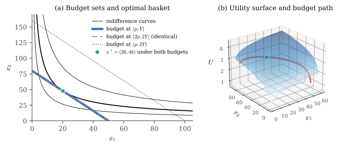
Figure 1
Figure 1: Cobb–Douglas, U=0.4log⁡x1+0.6log⁡x2U=0.4\log x_1+0.6\log x_2⁠, p=(40,25)p=(40,25)⁠, Y=2000Y=2000⁠. (a) The budget lines at (p,Y)(p,Y) and (2p,2Y)(2p,2Y) coincide, so the optimum x∗x^* is unchanged; doubling income alone (dotted) shifts the line out. (b) The utility surface, the budget path on it, and its highest point x∗x^*⁠.

3. Imposing the restriction

The restriction. Replace every pjp_j by λpj\lambda p_j and YY by λY\lambda Y in (1):

log⁡q1(λp,λY)=β0+∑j=1Jβjlog⁡(λpj)+βJ+1log⁡(λY)+u=β0+∑j=1Jβj(log⁡λ+log⁡pj)+βJ+1(log⁡λ+log⁡Y)+u=β0+∑j=1Jβjlog⁡pj+βJ+1log⁡Y+u⏟log⁡q1(p,Y)+(∑j=1Jβj+βJ+1)log⁡λ=log⁡q1(p,Y)+θlog⁡λ.(15)\begin{aligned} \log q_1(\lambda p,\lambda Y)&=\beta_0+\sum_{j=1}^J\beta_j\log(\lambda p_j)+\beta_{J+1}\log(\lambda Y)+u \\ &=\beta_0+\sum_{j=1}^J\beta_j(\log\lambda+\log p_j)+\beta_{J+1}(\log\lambda+\log Y)+u \\ &=\underbrace{\beta_0+\sum_{j=1}^J\beta_j\log p_j+\beta_{J+1}\log Y+u}_{\log q_1(p,Y)}+\Big(\sum_{j=1}^J\beta_j+\beta_{J+1}\Big)\log\lambda \\ &=\log q_1(p,Y)+\theta\log\lambda. && \htmlId{equation-15}{(15)} \end{aligned}

Homogeneity requires θlog⁡λ=0\theta\log\lambda=0 for all λ>0\lambda>0⁠. A product of two numbers is zero only if one of them is. Taking λ=2\lambda=2⁠, so that log⁡λ≠0\log\lambda\ne0⁠, shows that θ=0\theta=0 is necessary; conversely θ=0\theta=0 makes (15) hold for every λ\lambda⁠. Hence

homogeneity of degree zero⟺∑j=1Jβj+βJ+1=0.(16)\text{homogeneity of degree zero}\quad\Longleftrightarrow\quad \sum_{j=1}^J\beta_j+\beta_{J+1}=0. \qquad \htmlId{equation-16}{(16)}

Solving the restriction. Any of the J+1J+1 slope coefficients can be eliminated; take the last price elasticity βJ\beta_J⁠:

∑j=1J−1βj+βJ+βJ+1=0βJ=−(∑j=1J−1βj+βJ+1).(17)\begin{aligned} \sum_{j=1}^{J-1}\beta_j+\beta_J+\beta_{J+1}&=0 \\ \beta_J&=-\Big(\sum_{j=1}^{J-1}\beta_j+\beta_{J+1}\Big). && \htmlId{equation-17}{(17)} \end{aligned}

Split the price sum in (1), substitute (17), expand and regroup:

log⁡q1=β0+∑j=1J−1βjlog⁡pj+βJlog⁡pJ+βJ+1log⁡Y+u=β0+∑j=1J−1βjlog⁡pj−(∑j=1J−1βj+βJ+1)log⁡pJ+βJ+1log⁡Y+u=β0+∑j=1J−1βjlog⁡pj−∑j=1J−1βjlog⁡pJ−βJ+1log⁡pJ+βJ+1log⁡Y+u=β0+∑j=1J−1βj (log⁡pj−log⁡pJ)+βJ+1 (log⁡Y−log⁡pJ)+ulog⁡q1=β0+∑j=1J−1βjlog⁡pjpJ+βJ+1log⁡YpJ+u.(18)\begin{aligned} \log q_1&=\beta_0+\sum_{j=1}^{J-1}\beta_j\log p_j+\beta_J\log p_J+\beta_{J+1}\log Y+u \\ &=\beta_0+\sum_{j=1}^{J-1}\beta_j\log p_j-\Big(\sum_{j=1}^{J-1}\beta_j+\beta_{J+1}\Big)\log p_J+\beta_{J+1}\log Y+u \\ &=\beta_0+\sum_{j=1}^{J-1}\beta_j\log p_j-\sum_{j=1}^{J-1}\beta_j\log p_J-\beta_{J+1}\log p_J+\beta_{J+1}\log Y+u \\ &=\beta_0+\sum_{j=1}^{J-1}\beta_j\,(\log p_j-\log p_J)+\beta_{J+1}\,(\log Y-\log p_J)+u \\ \log q_1&=\beta_0+\sum_{j=1}^{J-1}\beta_j\log\frac{p_j}{p_J}+\beta_{J+1}\log\frac{Y}{p_J}+u. && \htmlId{equation-18}{(18)} \end{aligned}

Imposing homogeneity means deflating every price and income by one of the prices: the regressors become J−1J-1 relative prices and one real income. Model (1) has K=J+2K=J+2 parameters; model (18) has 1+(J−1)+1=J+1=K−11+(J-1)+1=J+1=K-1⁠, one fewer, which is what one restriction should cost. The coefficients keep their meaning: βj\beta_j is still the elasticity with respect to pjp_j⁠, other nominal prices and YY held fixed.

Recovering β^J\hat{\beta}_J and its standard error. After OLS on (18), the missing elasticity comes from the restriction itself. Write b^R=(β^0,β^1,…,β^J−1,β^J+1)′\hat{b}_R=(\hat{\beta}_0,\hat{\beta}_1,\dots,\hat{\beta}_{J-1},\hat{\beta}_{J+1})'⁠, V^R\hat{V}_R its estimated covariance matrix, a=(0,−1,…,−1)′a=(0,-1,\dots,-1)' and S={1,…,J−1,J+1}S=\{1,\dots,J-1,J+1\}⁠:

β^J=−(∑j=1J−1β^j+β^J+1)=a′b^RVar⁡^(β^J)=a′V^Ra=∑j∈SVar⁡^(β^j)+2∑j,k∈S, j<kCov⁡^(β^j,β^k).(19)\begin{aligned} \hat{\beta}_J&=-\Big(\sum_{j=1}^{J-1}\hat{\beta}_j+\hat{\beta}_{J+1}\Big)=a'\hat{b}_R \\ \widehat{\operatorname{Var}}(\hat{\beta}_J)&=a'\hat{V}_Ra=\sum_{j\in S}\widehat{\operatorname{Var}}(\hat{\beta}_j)+2\sum_{j,k\in S,\ j<k}\widehat{\operatorname{Cov}}(\hat{\beta}_j,\hat{\beta}_k). && \htmlId{equation-19}{(19)} \end{aligned}

The covariances matter: summing the variances alone would be wrong.

Invariance to the numeraire. OLS on (18) minimises the sum of squared residuals of (1) subject to (16). That problem does not depend on which coefficient is eliminated, so the estimates are identical whichever price deflates. In the simulation below, the three numeraires give coefficients that differ by at most 6×10−156\times 10^{-15}⁠.

The trade-off, step by step. Stack (1) as y=Xβ+uy=X\beta+u with β=(β0,…,βJ+1)′\beta=(\beta_0,\dots,\beta_{J+1})'⁠, and write the restriction as c′β=0c'\beta=0 with c=(0,1,…,1)′c=(0,1,\dots,1)'⁠. Let β^U=(X′X)−1X′y\hat{\beta}_U=(X'X)^{-1}X'y⁠, θ^=c′β^U\hat{\theta}=c'\hat{\beta}_U⁠, h=(X′X)−1ch=(X'X)^{-1}c and m=c′(X′X)−1cm=c'(X'X)^{-1}c⁠. Restricted least squares minimises (y−Xβ)′(y−Xβ)(y-X\beta)'(y-X\beta) subject to c′β=0c'\beta=0⁠:

FOC of (y−Xβ)′(y−Xβ)+2ν c′β:−2X′(y−Xβ^R)+2νc=0X′Xβ^R=X′y−νcβ^R=β^U−νhimpose c′β^R=0:0=θ^−νm⟹ν=θ^/mβ^R=β^U−θ^m h.(20)\begin{aligned} \text{FOC of } (y-X\beta)'(y-X\beta)+2\nu\,c'\beta:\quad -2X'(y-X\hat{\beta}_R)+2\nu c&=0 \\ X'X\hat{\beta}_R&=X'y-\nu c \\ \hat{\beta}_R&=\hat{\beta}_U-\nu h \\ \text{impose } c'\hat{\beta}_R=0:\quad 0=\hat{\theta}-\nu m\quad&\Longrightarrow\quad \nu=\hat{\theta}/m \\ \hat{\beta}_R&=\hat{\beta}_U-\frac{\hat{\theta}}{m}\,h. && \htmlId{equation-20}{(20)} \end{aligned}

This is the OLS estimator of (18), written in terms of (1). With Var(β^U)=σ2(X′X)−1\mathrm{Var}(\hat{\beta}_U)=\sigma^2(X'X)^{-1}⁠, Cov(β^U,θ^)=Var(β^U) c=σ2h\mathrm{Cov}(\hat{\beta}_U,\hat{\theta})=\mathrm{Var}(\hat{\beta}_U)\,c=\sigma^2h and Var(θ^)=σ2m\mathrm{Var}(\hat{\theta})=\sigma^2m⁠. Take the coefficient β1\beta_1 (first element of hh⁠: h1h_1), conditional on XX⁠:

β^1,R=β^1,U+δ θ^,δ≡−h1m=−Cov⁡(β^1,U,θ^)Var⁡(θ^)(21)E(β^1,R)=β1+δ θ(22)Var⁡(β^1,R)=Var⁡(β^1,U)+δ2Var⁡(θ^)+2δ Cov⁡(β^1,U,θ^)=Var⁡(β^1,U)+Cov⁡(β^1,U,θ^)2Var⁡(θ^)−2 Cov⁡(β^1,U,θ^)2Var⁡(θ^)=(1−ρ2) Var⁡(β^1,U),ρ≡corr⁡(β^1,U,θ^).(23)\begin{aligned} \hat{\beta}_{1,R}&=\hat{\beta}_{1,U}+\delta\,\hat{\theta},\qquad \delta\equiv-\frac{h_1}{m}=-\frac{{\operatorname{Cov}}(\hat{\beta}_{1,U},\hat{\theta})}{{\operatorname{Var}}(\hat{\theta})} && \htmlId{equation-21}{(21)} \\ E(\hat{\beta}_{1,R})&=\beta_1+\delta\,\theta && \htmlId{equation-22}{(22)} \\ {\operatorname{Var}}(\hat{\beta}_{1,R})&={\operatorname{Var}}(\hat{\beta}_{1,U})+\delta^2{\operatorname{Var}}(\hat{\theta})+2\delta\,{\operatorname{Cov}}(\hat{\beta}_{1,U},\hat{\theta}) \\ &={\operatorname{Var}}(\hat{\beta}_{1,U})+\frac{{\operatorname{Cov}}(\hat{\beta}_{1,U},\hat{\theta})^2}{{\operatorname{Var}}(\hat{\theta})}-2\,\frac{{\operatorname{Cov}}(\hat{\beta}_{1,U},\hat{\theta})^2}{{\operatorname{Var}}(\hat{\theta})} \\ &=(1-\rho^2)\,{\operatorname{Var}}(\hat{\beta}_{1,U}),\qquad \rho\equiv\operatorname{corr}(\hat{\beta}_{1,U},\hat{\theta}). && \htmlId{equation-23}{(23)} \end{aligned}

If H0H_0 is true (θ=0\theta=0), imposing the restriction removes the share ρ2\rho^2 of the variance (23) at no cost. If it is false, the estimator is shifted by δθ\delta\theta (22). Both effects come from the same source: how strongly β^1\hat{\beta}_1 co-moves with θ^\hat{\theta}⁠.

A common intuition says that the gain is largest when prices move together because of common inflation. This intuition is wrong. A common inflation factor raises the pairwise correlations among nominal prices, but it adds variation only along the direction (1,…,1)(1,\dots,1)⁠: exactly the direction that identifies θ\theta⁠, which leaves relative prices unchanged. It therefore lowers ρ\rho⁠, and imposing the restriction then buys almost no precision. Yet δ\delta⁠, and hence the bias when H0H_0 is false, is unchanged in our design (Figure 3). The gain is large when the price level varies little independently of relative prices and real income: a single cross-section, a period of stable inflation, or a price level that trends together with real income.

Identification. The restriction creates no identifying variation. In (18), βj\beta_j (j<Jj<J) is identified only by variation in relative prices across regions or over time. If prices move only through common inflation, log⁡(pj/pJ)\log(p_j/p_J) is constant and (18) cannot be estimated; in (1) only θ\theta is then identified.

4. Testing the restriction

The hypotheses are H0: ∑j=1Jβj+βJ+1=0H_0:\ \sum_{j=1}^J\beta_j+\beta_{J+1}=0 against H1: ∑j=1Jβj+βJ+1≠0H_1:\ \sum_{j=1}^J\beta_j+\beta_{J+1}\ne0⁠, in the unrestricted model (1). Let s2=SSRU/(n−K)s^2=\mathrm{SSR}_U/(n-K)⁠, so that V^U=s2(X′X)−1\hat{V}_U=s^2(X'X)^{-1}⁠.

1. Student tt on a linear combination.

θ^=c′β^U=∑j=1Jβ^j+β^J+1se⁡(θ^)2=c′V^Uc=s2m=∑j=1J+1Var⁡^(β^j)+2∑1≤j<k≤J+1Cov⁡^(β^j,β^k)t=θ^se⁡(θ^) ∼ tn−Kunder H0 (normal errors).(24)\begin{aligned} \hat{\theta}&=c'\hat{\beta}_U=\sum_{j=1}^J\hat{\beta}_j+\hat{\beta}_{J+1} \\ {\operatorname{se}}(\hat{\theta})^2&=c'\hat{V}_Uc=s^2m=\sum_{j=1}^{J+1}\widehat{\operatorname{Var}}(\hat{\beta}_j)+2\sum_{1\le j<k\le J+1}\widehat{\operatorname{Cov}}(\hat{\beta}_j,\hat{\beta}_k) \\ t&=\frac{\hat{\theta}}{{\operatorname{se}}(\hat{\theta})}\ \sim\ t_{n-K}\quad\text{under }H_0\text{ (normal errors).} && \htmlId{equation-24}{(24)} \end{aligned}

2. Reparametrisation. Rewrite (1) so that θ\theta becomes a coefficient. Start from (1) with the price sum split, write log⁡pj=log⁡(pj/pJ)+log⁡pJ\log p_j=\log(p_j/p_J)+\log p_J and log⁡Y=log⁡(Y/pJ)+log⁡pJ\log Y=\log(Y/p_J)+\log p_J⁠, and collect the terms in log⁡pJ\log p_J⁠:

log⁡q1=β0+∑j=1J−1βjlog⁡pj+βJlog⁡pJ+βJ+1log⁡Y+u=β0+∑j=1J−1βj(log⁡pjpJ+log⁡pJ)+βJlog⁡pJ+βJ+1(log⁡YpJ+log⁡pJ)+u=β0+∑j=1J−1βjlog⁡pjpJ+βJ+1log⁡YpJ+(∑j=1J−1βj+βJ+βJ+1)log⁡pJ+ulog⁡q1=β0+∑j=1J−1βjlog⁡pjpJ+βJ+1log⁡YpJ+θlog⁡pJ+u.(25)\begin{aligned} \log q_1&=\beta_0+\sum_{j=1}^{J-1}\beta_j\log p_j+\beta_J\log p_J+\beta_{J+1}\log Y+u \\ &=\beta_0+\sum_{j=1}^{J-1}\beta_j\Big(\log\frac{p_j}{p_J}+\log p_J\Big)+\beta_J\log p_J+\beta_{J+1}\Big(\log\frac{Y}{p_J}+\log p_J\Big)+u \\ &=\beta_0+\sum_{j=1}^{J-1}\beta_j\log\frac{p_j}{p_J}+\beta_{J+1}\log\frac{Y}{p_J}+\Big(\sum_{j=1}^{J-1}\beta_j+\beta_J+\beta_{J+1}\Big)\log p_J+u \\ \log q_1&=\beta_0+\sum_{j=1}^{J-1}\beta_j\log\frac{p_j}{p_J}+\beta_{J+1}\log\frac{Y}{p_J}+\theta\log p_J+u. && \htmlId{equation-25}{(25)} \end{aligned}

Model (25) is (1) with the same fit and the same coefficients β0,…,βJ−1,βJ+1\beta_0,\dots,\beta_{J-1},\beta_{J+1}⁠; it reduces to (18) when θ=0\theta=0⁠. Regressing log⁡q1\log q_1 on the regressors of (18) plus log⁡pJ\log p_J⁠, the coefficient on log⁡pJ\log p_J is θ^\hat{\theta}⁠, its standard error is se(θ^)\mathrm{se}(\hat{\theta})⁠, and its usual tt statistic is (24). Any regression software then reports the test and the confidence interval for θ\theta directly.

3. Fisher test, and why F=t2F=t^2⁠. Let eU=y−Xβ^Ue_U=y-X\hat{\beta}_U⁠, with X′eU=0X'e_U=0⁠. By (20), y−Xβ^R=eU+(θ^/m)Xhy-X\hat{\beta}_R=e_U+(\hat{\theta}/m)Xh⁠, and h′X′Xh=c′(X′X)−1c=mh'X'Xh=c'(X'X)^{-1}c=m⁠:

SSRR=eU′eU+2θ^mh′X′eU+θ^2m2h′X′Xh=SSRU+θ^2m(26)F=(SSRR−SSRU)/1SSRU/(n−K)=θ^2/ms2=θ^2se⁡(θ^)2=t2 ∼ F(1,n−K)  under H0.(27)\begin{aligned} \mathrm{SSR}_R&=e_U'e_U+2\frac{\hat{\theta}}{m}h'X'e_U+\frac{\hat{\theta}^2}{m^2}h'X'Xh =\mathrm{SSR}_U+\frac{\hat{\theta}^2}{m} && \htmlId{equation-26}{(26)} \\ F&=\frac{(\mathrm{SSR}_R-\mathrm{SSR}_U)/1}{\mathrm{SSR}_U/(n-K)}=\frac{\hat{\theta}^2/m}{s^2}=\frac{\hat{\theta}^2}{{\operatorname{se}}(\hat{\theta})^2}=t^2\ \sim\ F(1,n-K)\ \text{ under }H_0. && \htmlId{equation-27}{(27)} \end{aligned}

The large-sample versions are W=n(SSRR−SSRU)/SSRUW=n(\mathrm{SSR}_R-\mathrm{SSR}_U)/\mathrm{SSR}_U (Wald) and LR=nlog⁡(SSRR/SSRU)LR=n\log(\mathrm{SSR}_R/\mathrm{SSR}_U) (likelihood ratio), both χ12\chi^2_1 under H0H_0⁠, with W≥LRW\ge LR⁠.

Reading the result. Not rejecting H0H_0 does not prove homogeneity: it means only that the data cannot distinguish θ\theta from zero at the chosen level. The confidence interval θ^±tn−K,0.975 se(θ^)\hat{\theta}\pm t_{n-K,0.975}\,\mathrm{se}(\hat{\theta}) is the informative object: it says which degrees of money illusion the data rule out. Applied work on complete demand systems has rejected homogeneity strikingly often (Deaton and Muellbauer, 1980). Laitinen (1978) showed that much of this comes from asymptotic tests, which over-reject badly when the number of equations is large relative to the sample, and derived the exact finite-sample distribution of the test statistic.

5. Simulation

Design. J=3J=3 goods, 5050 regions ×\times 1010 periods (n=500n=500). Log prices are log⁡pjrt=πt+μjr+ϵjrt\log p_{jrt}=\pi_t+\mu_{jr}+\epsilon_{jrt}⁠: common inflation πt∼N(0,0.22)\pi_t\sim N(0,0.2^2)⁠, regional price levels μjr∼N(0,0.152)\mu_{jr}\sim N(0,0.15^2)⁠, shocks ϵjrt∼N(0,0.052)\epsilon_{jrt}\sim N(0,0.05^2)⁠. Log income is log⁡Yrt=log⁡2000+πt+ωrt\log Y_{rt}=\log 2000+\pi_t+\omega_{rt} with ωrt∼N(0,0.32)\omega_{rt}\sim N(0,0.3^2)⁠, and u∼N(0,0.22)u\sim N(0,0.2^2) (seed 20261015). Under H0H_0⁠: β=(−0.6, 0.2, 0.1, 0.3)\beta=(-0.6,\,0.2,\,0.1,\,0.3)⁠, so θ=0\theta=0⁠. Under H1H_1⁠, only the income elasticity changes, to 0.40.4⁠, so θ=0.1\theta=0.1⁠; the same uu is used for both, which makes the H0H_0 and H1H_1 columns directly comparable.

Table 1: Estimates on the data generated under H0H_0 (standard errors in parentheses).

TrueUnrestricted (1)Restricted (18)Reparametrised (25)
β0\beta_0 (constant)1.0000.872 (0.218)0.855 (0.217)0.872 (0.218)
β1\beta_1 (log⁡p1\log p_1)-0.600-0.594 (0.050)-0.586 (0.048)-0.594 (0.050)
β2\beta_2 (log⁡p2\log p_2)0.2000.195 (0.049)0.205 (0.046)0.195 (0.049)
β3\beta_3 (log⁡p3\log p_3)0.1000.053 (0.048)0.064a (0.045)0.053b (0.048)
β4\beta_4 (log⁡Y\log Y)0.3000.315 (0.029)0.317 (0.028)0.315 (0.029)
θ=∑jβj+β4\theta=\sum_j\beta_j+\beta_40.000-0.032 (0.050)0 (imposed)-0.032c (0.050)
SSR18.699418.715418.6994
Parameters545

a Recovered by (19). b Recovered as θ^−β^1−β^2−β^4\hat{\theta}-\hat{\beta}_1-\hat{\beta}_2-\hat{\beta}_4⁠. c Coefficient of log⁡p3\log p_3 in (25).

Estimates and tests. In Table 1, the reparametrised regression (25) reproduces the unrestricted coefficients and delivers θ^\hat{\theta} as an ordinary coefficient. Imposing the restriction shrinks the standard error of β^1\hat{\beta}_1 from 0.0500.050 to 0.0480.048 and that of β^3\hat{\beta}_3 from 0.0480.048 to 0.0450.045⁠. The gains are modest, as (23) predicts with ρ^=0.25\hat{\rho}=0.25 in this sample. In Table 2, FF and t2t^2 agree to 2×10−132\times 10^{-13}⁠, as (27) requires. Under H0H_0 the test does not reject (p=0.51p=0.51). Under H1H_1 it does not reject either (p=0.17p=0.17), yet the interval [−0.030,0.165][-0.030,0.165] contains the true θ=0.1\theta=0.1⁠. This is the warning of Section 4 in numbers: non-rejection is not evidence of homogeneity.

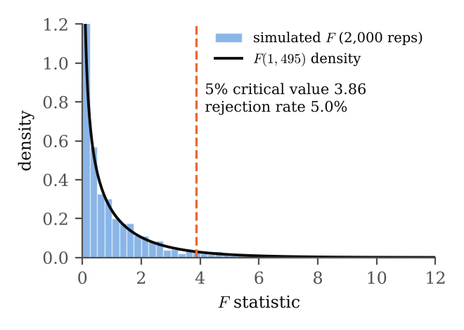
Size and power. Over 2,0002{,}000 samples drawn under H0H_0⁠, the FF statistic follows its F(1,495)F(1,495) distribution (Figure 2; Kolmogorov–Smirnov p=0.53p=0.53). The test rejects in 5.0%5.0\% of samples, with a Monte Carlo standard error of 0.50.5 points. At θ=0.1\theta=0.1⁠, power is 0.600.60 with n=500n=500 and 0.980.98 with n=2,000n=2{,}000 (Figure A.1, appendix).

Table 2: Tests of H0:θ=0H_0:\theta=0 on the data generated under H0H_0 and under H1H_1 (same regressors and errors).

H0H_0⁠: θ=0\theta=0H1H_1⁠: θ=0.1\theta=0.1
θ^\hat{\theta}-0.03230.0677
se(θ^)\mathrm{se}(\hat{\theta})0.04950.0495
tt-0.65171.3683
t2t^20.42471.8723
FF from SSRs0.42471.8723
pp-value (tt and FF)0.5150.172
95% CI for θ\theta[-0.130, 0.065][-0.030, 0.165]
Wald / LR (χ12\chi^2_1)0.429 / 0.4291.891 / 1.888
Figure 2
Figure 2: Size: FF over 2,0002{,}000 samples under H0H_0⁠, and the F(1,495)F(1,495) density.
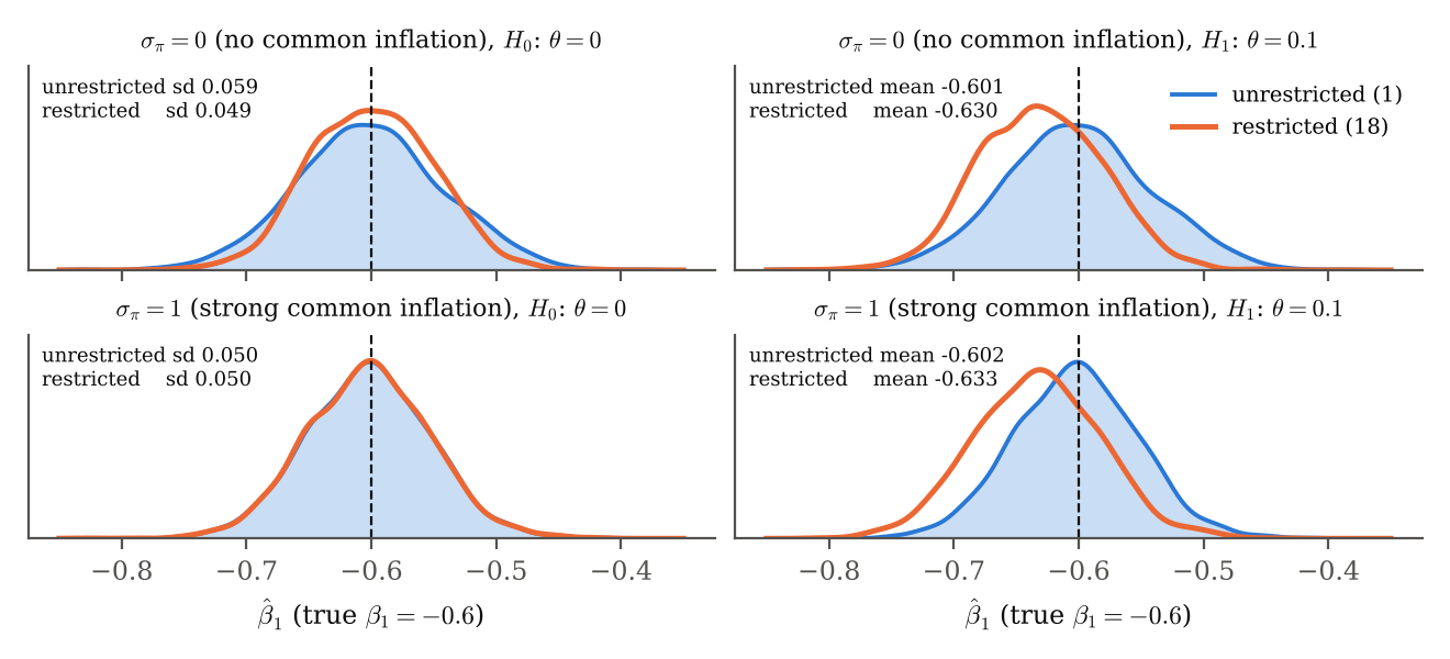
Figure 3
Figure 3: Sampling distribution of β^1\hat{\beta}_1⁠, unrestricted (1) and restricted (18), n=500n=500⁠, 2,0002{,}000 samples. Top row: no common inflation. Bottom row: strong common inflation, where corr(log⁡p1,log⁡p2)=0.97\mathrm{corr}(\log p_1,\log p_2)=0.97⁠.

The cost of imposing. Figure 3 illustrates (22) and (23). Without common inflation, nominal prices are uncorrelated (corr=0.00\mathrm{corr}=0.00), yet imposing a true restriction cuts the standard deviation of β^1\hat{\beta}_1 from 0.0590.059 to 0.0490.049 (ratio 0.830.83⁠; (23) gives 0.830.83). With strong common inflation, prices are highly correlated and the gain vanishes (ratio 1.001.00). If the restriction is false, the restricted estimator is shifted by −0.029-0.029 and −0.031-0.031 relative to the unrestricted one ((22) gives −0.031-0.031 and −0.031-0.031), while the unrestricted estimator stays centred on −0.6-0.6⁠. The design that makes imposition worthwhile is also the one in which the test is weakest: se(θ^)\mathrm{se}(\hat{\theta}) is 0.1060.106 without common inflation against 0.0110.011 with it. Precisely when imposing homogeneity buys precision, the data say least about whether it holds.

Conclusion. Zero-degree homogeneity is not an assumption on preferences but a consequence of the budget constraint, and in a log-linear demand it reduces to one linear restriction, θ=0\theta=0⁠. Test it as the coefficient on log⁡pJ\log p_J in the reparametrised regression (25) and report its confidence interval. Impose it knowing that the gain (23) and the risk (22) are governed by the same correlation between β^j\hat{\beta}_j and θ^\hat{\theta}⁠.

References

Deaton, A. and J. Muellbauer (1980). Economics and Consumer Behavior. Cambridge: Cambridge University Press.

LaFrance, J. T. (1986). The structure of constant elasticity demand models. American Journal of Agricultural Economics 68(3), 543–552.

Laitinen, K. (1978). Why is demand homogeneity so often rejected? Economics Letters 1(3), 187–191.

Stone, R. (1954). Linear expenditure systems and demand analysis: an application to the pattern of British demand. Economic Journal 64(255), 511–527.

Appendix: power of the test
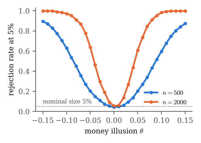
Figure A.1
Figure A.1: Power: rejection rate of the 5% FF test as a function of θ\theta (1{,}000 samples per sample size; common random numbers across θ\theta).
  1. This note draws on working documents and calculations I prepared during my PhD to understand these concepts. I sometimes use these materials in my econometrics courses and share them here for teaching and learning. ↩