The Household Demand for Leisure, the Price of Time and the Full Cost of Children: A Structural Model and Evidence from the PSID
Manuscript references include the physical PDF page. If a PDF does not display or your reader ignores the page number, use the source-page viewer.
Research question
What do children cost when parental childcare time is partly productive and partly experienced as leisure?
Children cost their parents money and time, and neither cost is observed. Children’s consumption is pooled with parents’ consumption in household expenditure data. Childcare hours are observed but cannot all be counted as a cost, because parents may draw leisure-like utility from them (process benefits).
The paper asks how both components, and their sum (the full cost of children), can be recovered from observed behavior without assuming that an hour of childcare is worth the parent’s wage.
Research contribution
An endogenous price of parental time, carried through to the full cost of children
- Time cost of children. Existing measures value parental time at the market wage or at the price of equivalent services (Gustafsson & Kjulin, 1994; Apps & Rees, 2001; Colombino, 2000; Bradbury, 2008). Here the price of parental childcare time is a shadow price recovered from behavior; wage valuation is the special case .
- Cost-of-children methods. The Rothbarth logic is applied to time rather than goods. The adult good is the parent’s full leisure, and resources are measured by full expenditure. Unlike Bargain & Donni (2012) and Bargain, Donni & Hentati (2022), no data on singles are needed. Unlike Dunbar, Lewbel & Pendakur (2013), no strong parametric restriction is placed on preferences across individuals.
- Process benefits. Graham & Green (1984), Kerkhofs & Kooreman (2003) and Gørtz (2011) study process benefits in home production. Cosaert & Hennebel (2023) show that childcare process benefits are only set-identified by revealed preference. This paper obtains point identification from the substitution between parental and purchased care (Reid’s 1934 third-party criterion) and maps it into a cost of children.
Non-technical overview
Valuing parental time to measure the full cost of children
Pricing a childcare hour at the wage presumes two things: the parent can freely trade that hour against paid work, and the hour is pure work, neither more nor less pleasant than a job.
The paper drops the second presumption. Following Reid’s criterion, the productive part of childcare is the part a nanny or a daycare could supply instead. Couples’ choices reveal what that part is worth. When wages change, couples shift between their own care hours and purchased care, and the rate at which one parental hour replaces paid care is its productive value. Whatever remains of the wage is the value of the hour as leisure.
The paper then infers how much of the family’s spending goes to children by comparing parents’ leisure—including the part of childcare they experience as leisure—with that of comparable childless couples. This comparison assumes that parenthood changes neither adults’ preferences for leisure nor how they share the resources left for themselves. Differences in leisure can then reveal resources devoted to children, rather than changes in tastes or redistribution between spouses. After accounting for the time cost of childcare, the model recovers the monetary cost of children.
Example. A mother in the sample earns $29.48 an hour on average (Table 2). The benchmark estimate prices the productive part of her childcare hour at about $13. The remaining $16.50 is leisure-like value (Table 4, col. A). Across couples with one child, the median weekly time cost is $230. Pricing every hour at the wage would give $350, about 50% more (Table 6, rows A and A*).
View Abstract
We propose a novel approach to estimating the full cost of children — the sum of monetary and time costs — by endogenizing the price of parental time rather than assuming it is equal to the parents’ wage rate. In this approach, the price of time depends on how parents perceive their time with children, whether as a leisure-like activity or more as a labor-like activity. We then develop a simplified collective model of leisure demand for working couples, incorporating individual preferences and childcare technology, and estimate it using 2019 PSID data. This allows us to recover the price of parental time and the full cost of children. We find that mothers perceive 44% of their childcare time as labor, compared to 35% for fathers. Our results also highlight that a substantial portion of the full cost of children is non-monetary.
Economic model
A collective model in which the wage splits into two shadow prices
Couple. Each spouse has preferences over:
- own leisure ,
- childcare time ,
- own consumption ,
- children’s consumption .
Decisions are Pareto-efficient.
Childcare technology. The function is the minimum purchased care needed, given parental hours, to meet the childcare requirement, so that and . It does not describe the production of child quality. It describes only how far parental time substitutes for market care.
Decentralization (Proposition 1). Each childcare hour is split into a productive component and a process-benefit component. Their prices sum to the wage, like Lindahl prices:
View details
The couple first minimizes the cost of meeting the childcare requirement:
View details
and then shares the remaining resources between the spouses and the children.
Cost of children. The time cost is shadow-valued parental time plus purchased care. The monetary cost is . The full cost is .
View details
With linear (Assumption A.1), full leisure is . The leisure-like share of childcare is counted as leisure, and only is counted as work.
Identification
Prices from substitution with paid care and children's consumption from full-leisure Engel curves
Step 1: the price of parental time (Propositions 2–3, Corollary 4).
- Interior regime (). The wage responses of identify the gradient of . At the optimum, the shadow price equals the marginal rate of technical substitution between a parental hour and purchased care, .
- Corner regime (). Only the ratio is identified.
- Resolving the corner. Under A.1, depends only on own childcare time, so it extends to the corner by continuity and the corner multiplier is identified.
- Testable implication. Childcare choices do not depend on non-labor income.
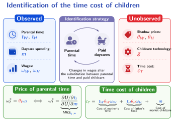
The slide uses for the wage , and for .
Step 2: the monetary cost (Proposition 6).
Two assumptions make the full-leisure demand the same for parents and non-parents:
is therefore estimated on childless couples and inverted for parents:
View details
This requires only local invertibility of one spouse’s Engel curve. It is robust to unmodelled interactions such as altruism, public goods or home production, provided children affect behavior only through . Under the weaker Similarity Across Types condition (A.2′), identification rests instead on the curvature of .
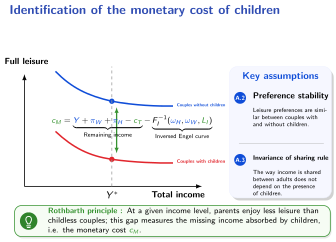
The slide uses for the wage , and for . The utility-profit terms in this general-model diagram are zero under the linear process-benefit specification used for estimation.
Econometric model & methods
Two recursive stages that mirror the two identification steps
Stage 1: couples with children, maximum likelihood.
- The time cost is Generalized Leontief in the shadow prices :
View details
- Shephard’s lemma gives two linear childcare-time equations and a Tobit equation for purchased care.
- The errors are jointly normal, and are estimated as free parameters.
View details
The estimated system is equations (9)–(12), manuscript PDF page 29; the two time equations are uncensored and purchased care is Tobit-censored. The theoretical corner switches shadow prices by a common multiplier, but this regime switch is omitted from the time equations in estimation (PDF page 32). View equations and estimation discussion.
Stage 2: all couples, three-stage least squares.
- Full leisure is built as .
- Each spouse’s full leisure is quadratic in remaining full expenditure , with or without demographic shifts (SAT).
- The monetary cost is specified as .
- Instruments are the stage-1 predicted time cost and, for full expenditure, non-labor income and its square.
Without SAT — preference stability (equations 15–16).
View details
With SAT — Similarity Across Types (equations 17–18). SAT leaves the slope of each full-leisure Engel curve invariant across parental status while permitting demographic level shifts.
View details
Data & sources
PSID 2019: hours of care and dollars of paid care for the same couples
- Survey. Panel Study of Income Dynamics, 2019 wave (9,569 households). It is one of the few surveys that records parental childcare time, childcare expenditure and wages for the same households.
- Sample. Dual-earner, non-student, heterosexual couples aged 22–50. Couples with children have at most two children and a youngest child aged six or under. The sample has 825 couples: 463 with children and 362 without (Table 2).
- Childcare time. The PSID question includes passive supervision. Reported hours are rescaled to match ATUS primary-childcare averages, with a transformation that preserves zeros:
View details
Mean childcare falls from 35.1 to 9.7 h/week for fathers and from 53.7 to 19.0 h/week for mothers (Table 1).
- Leisure. Leisure is non-market time, .
- Paid care. Purchased childcare is 2018 annual spending divided by 52: $100/week on average, with 35% zeros (Table 1).
- Robustness. The analysis is replicated on the 2017 wave (Tables A.1–A.3).
| Variables | Mean | SD | Min | Median | Max | Zero share |
|---|---|---|---|---|---|---|
| Father PSID childcare, original | 35.12 | 39.72 | 0.00 | 20.00 | 168.00 | 0.02 |
| Mother PSID childcare, original | 53.65 | 46.39 | 0.00 | 40.00 | 168.00 | 0.01 |
| Father PSID childcare, adjusted | 9.66 | 20.65 | 0.00 | 0.91 | 115.17 | 0.02 |
| Mother PSID childcare, adjusted | 18.97 | 28.45 | 0.00 | 6.63 | 116.91 | 0.01 |
| Childcare expenditure, $/week | 99.91 | 127.46 | 0.00 | 49.96 | 769.23 | 0.35 |
| Variables | Without children | With children |
|---|---|---|
| Father adjusted childcare, hours/week | 0.00 (0.00) | 9.66 (20.65) |
| Mother adjusted childcare, hours/week | 0.00 (0.00) | 18.97 (28.45) |
| Childcare expenditure, $/week | 0.00 (0.00) | 99.91 (127.46) |
| Number of children | 0.00 (0.00) | 1.56 (0.50) |
| Child under 3 | 0.00 (0.00) | 0.74 (0.44) |
| Father leisure, hours/week | 125.33 (12.28) | 114.76 (22.32) |
| Mother leisure, hours/week | 130.79 (12.30) | 115.49 (28.62) |
| Father wage, $/hour | 30.71 (44.51) | 31.97 (25.89) |
| Mother wage, $/hour | 24.36 (16.36) | 29.48 (26.25) |
| Full expenditure, $000 | 5.52 (4.15) | 6.31 (4.25) |
| Father education, years | 14.24 (2.26) | 14.38 (2.39) |
| Mother education, years | 14.84 (2.10) | 15.15 (1.87) |
| Father age, years | 36.71 (7.82) | 34.21 (5.33) |
| Mother age, years | 35.58 (7.84) | 32.88 (5.04) |
| Couples | 362 | 463 |
Table 1: SD = standard deviation; zero share = proportion of zeros. Table 2: means with standard deviations in parentheses; hours per week, hourly wages in dollars, full expenditure in thousands of dollars per week, education and age in years. Full expenditure includes goods, services and leisure valued at spouses’ wages.
Provider
PSID, Institute for Social Research, University of Michigan
Official provider site
Access
2019 Panel Study of Income Dynamics
Open PSID Data Center information
Documentation
Exact data used
2019 PSID Family File universe (9,569 households) restricted to 825 dual-earner couples aged 22–50: 463 with children and 362 childless. Measures include wages, work hours, broad retrospective childcare time, external childcare spending, education, ages and household expenditures.
Access conditions: Registration and a customized Data Center extract are required; no raw or customized extract is redistributed.
Results & limits
Time valuation and cost estimates
| PSID 2019 | Benchmark | Range across specifications |
|---|---|---|
| Labor-like share of mothers’ childcare, (Table 4) | 0.44 (0.26) | 0.30–0.44 |
| Labor-like share of fathers’ childcare, (Table 4) | 0.35 (0.21) | 0.20–0.35 |
| Time cost, one child, $/week: median / mean (Table 6) | 230 / 430 | 170–570 / 290–810 |
| … same, with time priced at the wage (Table 6, A*) | 350 / 930 | — |
| Monetary cost, one child, $/week: median / mean (Table 6) | 480 / 770 | 430–890 / 770–1,210 |
Standard errors are reported in parentheses.
Main findings
- Between 56% and 70% of mothers’ childcare time, and between 65% and 80% of fathers’, is leisure-like (Table 4).
- The 2017 wave also yields , with and (Table A.3).
- Parental time inputs are complements ().
- Full leisure rises by 3.2 hours (men) and 4.4 hours (women) per extra $1,000 of weekly full expenditure (Table 5).
- The model’s exclusion restrictions are not rejected: non-labor income can be excluded from the full-leisure equations (p = 0.98), and the monetary-cost parameters are equal across spouses (p = 0.98).
- Parental childcare is valued at about 30–50% of the wage.
View exclusion tests and median-wage uncertainty, PDF page 39.
LIMITS
- Results apply to dual-earner couples with young children and capture short-run costs only; career costs are excluded.
- The PSID childcare measure includes passive care. The ATUS rescaling reshapes its distribution, and the time cost is sensitive to it (row E).
- Rationing of formal care or unobserved fixed costs may bias downward.
- Full leisure responds weakly to resources, so the monetary cost is imprecise. At median wages it is $566 (s.e. 286), against $344 (s.e. 120) for the time cost.
- The Generalized Leontief cost function is not globally consistent, and the zero-paid-care regime is not modelled in estimation.
Presentation
Documents, citation, and contact
Manuscript and related material
- Current manuscript — PDFVersion October 4, 2026
- Conference slides — PDFAugust 17, 2026 · 42 pages
- Tables and figures: accessible source-page viewerUse this viewer if your PDF reader ignores page fragments.
- Code & DataResearch code will be made available after publication of the paper.
Questions, seminar invitations, or collaboration ideas are welcome.
Contact Anderson Vil about this paper